This website uses Cookies. Click Accept to agree to our website's cookie use as described in our Privacy Policy. Click Preferences to customize your cookie settings.
Turn on suggestions
Auto-suggest helps you quickly narrow down your search results by suggesting possible matches as you type.
Showing results for
- Looker
- Looker Forums
- Modeling
- A (Hitchhiker's) Guide to Query Performance in Loo...
Topic Options
- Subscribe to RSS Feed
- Mark Topic as New
- Mark Topic as Read
- Float this Topic for Current User
- Bookmark
- Subscribe
- Mute
- Printer Friendly Page
Solved


 LinkedIn
 Twitter
Post Options
- Mark as New
- Bookmark
- Subscribe
- Mute
- Subscribe to RSS Feed
- Permalink
- Report Inappropriate Content
Reply posted on
--/--/---- --:-- AM
Post Options
- Mark as New
- Bookmark
- Subscribe
- Mute
- Subscribe to RSS Feed
- Permalink
- Report Inappropriate Content
Problem: You’ve written alot of very nice LookML, but your data is >20TB and queries take forever. This isn’t fun, and your business users are complaining - a tragedy! Never fear, this post is here.
Prerequisites:
- Be familiar with the doc “How Looker Generates SQL”
- Understand basic SQL syntax (eg what each clause is, basic SQL functions, etc)
- Have at least developer permissions in Looker (with SQL Runner access)
- Be familiar with LookML terms and concepts
Post Context:
This is adapted from DCL’s internal SME (Subject Matter Expert) curricula; similar to “Knowledge Drops”, the information here may be highly Looker specific and at some point become out of date. Additionally, the information here should be thought of as a sort of ELI5, not an in depth description of how things work. The goal is to provide a “quick and dirty” guide to facilitate troubleshooting query performance, not something that is technically comprehensive - for that, you may find better mileage elsewhere.
What this covers:
- 1: Fundamental SQL Concepts
- 2: Factors Impacting Query Performance
- 3: Tuning Strategies
In a later set of posts, I’ll cover how and why SQL Performance impacts Looker application performance and how this ties into more strategic things you can do as a Looker Admin or Developer to provide good experiences for your end-users.
Fundamental SQL Concepts
Order of Operations

This may seem mundane and unimportant, but understanding the order of operations and what happens at each step is crucial in understanding why a query would be non-performant, and understanding what needs to be resolved to make it performant.
Understanding the shape of a query
One way to see how many rows of data are being queried over for each stage is to iteratively adjust the query like so:
-- 1: run with just the joins to see what is being queried at step 1
select count(*)
from <table>
<joins here>
-- 2: add where clause to see what is filtered out
<where clause>
-- 3: add the columns grouped by to the select, then add the group by.
<group by>
The count from 1 will tell you how large the joined dataset is. Count from 2, how much your where clause has helped reduce the ResultSet. Count from 3, how many rows the group by is reducing the query. Group bys are expensive, as we will touch on later.
Another way to get insight into what is happening at each query stage is to use EXPLAIN if your database supports it. See: https://help.looker.com/hc/en-us/articles/360023513514-How-to-Optimize-SQL-with-EXPLAIN
To illustrate this with an example, say we have 3 tables, each with 1k rows, and we query it with a where clause that filters out 1k rows, a group by that reduces the query by a further 1k rows, and a having clause that filters out 500 rows. When executed, that query will move through the OoO like so:
It’s important to note that most modern Databases can bring millions or even tens of millions of rows into memory quite quickly (although as tables grow past that this does not hold true) and return that resultset, however it’s usually what we do to those millions or hundreds of millions of rows that makes dataset size problematic. Using a few example queries to illustrate:
-
Simple select * of 500k rows > Most databases will return this fairly quickly
-
Simple select some number of columns of 500k rows > Similarly, most database return this just as quickly
-
Select sum(number) of 500k rows > This generally takes the database a bit longer, but not unreasonably. All the database has to do is add up the entire column, and since aggregates are not that expensive over medium-large size datasets this is fine
-
Select case when number over 500k rows > This query will generally take far longer, on the order of 10x previous queries, because the database has to perform a row by row transformation. While a case when or string function isn’t expensive at one row, over many rows it’s expense adds up.
Along similar lines, a LIMIT clause will do little to help decrease query runtime, because it happens at the final stage of the query, after the ResultSet has been brought together and all transformations in the select and aggregations in the group by completed. Query runtime is a function of the number of rows we are doing calculations over, not the number of rows returned to the user.
The query size estimator tool can be useful in understanding how much data is in the base datasets. However, Kb estimate does not necessarily correlate with query runtime because this doesn’t measure the amount of work the DB needs to perform, just the amount of raw data it needs to perform that work over from each table.
A few things regarding size to keep in mind:
-
What if the requested tables are so large, the DB cannot bring them into memory? The database will bring what it can into memory, then read the rest from disk. Reading from disk is much slower. This is where we would expect the size of a full, joined dataset in the FROM stage to cause a non-performant query.
-
How is this different with columnar databases? The database will only bring into memory what is needed in the select and where clauses. This is one reason why columnar databases are faster than row-oriented dbs when running queries over few columns but large numbers of rows -- as the columnar db is less likely to need to read from disk.
-
What if we are applying a limit in a derived table, then querying from that table? This is where a LIMIT clause can become beneficial, if the derived table is persisted. If your PDT limits the dataset, your outer query will be running over only the rows captured by the LIMIT. This benefit is lost if the derived table is not persisted, since the derived table will generate as a CTE.
Factors Impacting Query Performance
Factors
Primarily, three factors are responsible for the “expense” of a query. By expense, I mean how much work a database has to do to process a given query:
-
Size of the base datasets
-
Size of the dataset after joins
-
num cols * row number of joined dataset
-
-
Expense of the functions being performed on each row of data
There is another (unelaborated on) factor that you should consider as well: the computational power of your DB (and DB’s environment). With some dialects (especially more modern ones), throwing more DB resources at the problem can usually be a solution.
Rules of Thumb
-
COUNTs are free
-
Other Aggregate functions are relatively inexpensive
-
DISTINCT and GROUP BY are expensive
-
Adding columns adds expense (ncol * kbof_col)
-
Analytic / Window functions are expensive
-
String/Formatting/Labeling functions are inexpensive, but become expensive as row count of the dataset after joins rises
-
Aggregate functions over the same number of rows are very inexpensive in relation
-
-
Functions used to transform data in the WHERE clause are executed at every row
-
HAVING clause has less performance benefit than WHERE, since it occurs after the GROUP BY is executed and aggregation has occurred
Understanding Database Types (Columnar vs Row Store)
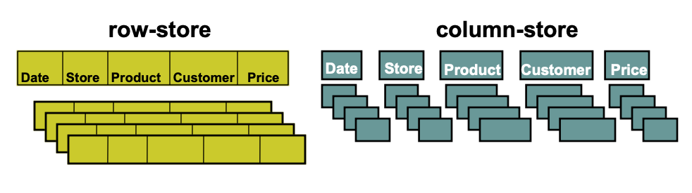
You may have heard the terms “Columnar” vs “Row Oriented” databases.This distinction is important to understand in the context of query performance, because it changes how a database loads a dataset into memory and thus how well it performs while scanning over large datasets with different query patterns.
For example, taking the table from above with columns Date, Store, Product, Customer, Price; if we were to execute the following query:
select Store, sum(price)
from Transactions
where Date = CURRENT_DATE()
group by 1
The query will execute on a row-store db like:
-
Load all rows in all 5 columns into memory; Date, Store, Product, Customer, Price
-
Scan the Date column with all 5 columns loaded to find rows matching CURRENT_DATE()
-
Perform the sum() on Price and the Group By on Store with all columns loaded
-
Finally, return the result set
While on a column-store db, the query will execute like:
-
Load only the Store, Price, and Date columns into memory
-
Scan the Date column
-
Group and Aggregate
-
Return resultset
In practice, this means columnar store databases excel at selecting a finite number of columns and performing aggregations over large datasets, but not so well at writing data to the DB (which is why we use MySQL as a backend db for the Looker application, not a columnar store db like BQ). Additionally, the more columns selected in a given query, the less well a columnar-store db performs in relation to a row-store oriented database.
Tuning
Partitions & Indexes
How do they work?
Technically, partitions and indexes are separate, and work differently, however in practice they are functionally very similar. Under the hood, indexes create pointers to sections of data in a table, and the index column, itself, is an ordered column in the table. When a query runs with a WHERE clause that evaluates the index column, the database refers to it’s list of pointers, limiting the number of rows the database has to bring into memory and execute other sections of the query over.
Partitioning is along the same lines, however it “shards” a table instead of just creating pointers. Similar to indexes, a condition in the WHERE clause that evaluates over the partition column will enable the query to leverage partitions. Note: each index and partition is table specific, so if your query joins multiple indexed/partitioned tables, each table’s index/partition column needs to be evaluated in the where clause.
Implementation
Individual dialects support different schemes for utilizing indexes/partitions. BigQuery, for example, allows the creation of either integer or time based partitions, and does not support use of indexes. Other databases, like Postgres, support the use of both. Partitions & indexes can be declared in SQL runner, depending on database dialect in LookML for PDTs, and in a DB’s console. In the context of BigQuery, leveraging partitions in Looker would look like:
-
Identify an appropriate column to use as the partition column
-
This can be an integer or date type column
-
The values in the column should have few enough values such that, each unique value rolls up many rows in the table.
-
-
Execute the partition by command. Each unique value in the partition column now becomes a partition.
-
For PDTs, partitions can be declared in LookML
-
https://docs.looker.com/reference/view-params/partition_keys
-
Looker will then execute a partition by command at table creation
-
-
At Looker-Query runtime, have Looker generate a WHERE condition that evaluates over the partition column
In Looker, the challenge will generally be in getting users to use partitions. There are a variety of strategies to use to ensure this happens, but they can range from content creators adding comments or notes to their content to the effect of “add x filter”, to a sql_always_where in LookML.
Aggregate & Rollup Tables
What are Aggregate & Rollup Tables?
Aggregate & Rollup tables are essentially just pre-aggregated tables; aggregating many rows of data into fewer rows, saving the result as a new table, then making that new table available to query instead of the original table(s). A scenario to illustrate:
Say users frequently evaluate the number and total value of sales by month. To get this result, they run the following query:
select date_month, count(distinct sale_id), sum(sale_price)
from sales
group by 1
The sales dataset is quite large, over 10 million rows, so the query takes quite some time to complete, and there are only 50 unique date_months (the field we’re grouping by) in the dataset. In this example, saving the original query as a new table, then having users query the new table instead of the raw table would mean user’s queries would only be over 50 rows instead of the full dataset’s 10 million, thus drastically reducing runtime (and cost depending on how the database handles billing). Aggregate & Rollup tables are fundamental concepts for query tuning, and can offer drastic performance improvements, depending on how they are implemented.
Implementation
In Looker, aggregate tables can easily be created via the following mechanisms:
-
Persistent Derived Tables (either sql or ndt): https://docs.looker.com/data-modeling/learning-lookml/derived-tables
-
Persistent Derived Tables with create process: https://docs.looker.com/reference/view-params/create_process
-
Aggregate Awareness: https://docs.looker.com/data-modeling/learning-lookml/aggregate_awareness
Each of the three has it’s own strengths and tradeoffs. See the table below:
| PDT | PDT with Create Process | Aggregate Awareness | |
| Pro |
|
|
|
| Con |
|
|
|
Data Transformations: ETL & PDTs
One of the strengths of LookML is how easy it is to define and codify data transformations on the fly. However, the weakness of this is that developers can easily cause Looker to generate non-performant SQL, specifically by doing many multiple data transformations in dimensions and measures, thus running them every time a dimension or measure is used.
To illustrate with an example: Say a dataset contains a column with “order codes” that denote the source of an order. These codes are not human readable, so a developer built out a dimension like this:
dimension: order_code_readable {
type: string
sql: case
when ${TABLE}.order_code = ‘A1’ then ‘Website’
when ${TABLE}.order_code = ‘A2’ then ‘Third Party’
when ${TABLE}.order_code = ‘B5’ then ‘In Person Sale’
end ;;
}
Every time a user runs a query using the dimension `order_code_readable`, and for every reference of that dimension in their other LookML constructs (sql_always_where, etc), Looker generates that case when, which must then calculate at every row. As we’ve touched on, this kind of relabeling at one row is fairly inexpensive, but over many rows it’s cost adds up. In the context of a query with many such transformations, or that is calculating over a large dataset, this will be expensive and inefficient.
Instead, a better way is to roll this transformation, along with any other similar transformations, up into a PDT (or even better make it a part of ETL), so that the transformation(s) build only once, and subsequent queries to the same table don’t need to perform the transformation every time they are ran. This rule of thumb also holds true with all other types of functions that evaluate row by row (string functions, window/analytical functions, etc). When possible, saving them to a table will have performance benefit, which depending on a variety of factors, can be significant.
TLDR
- Reduce the number of rows pulled be a query as early as possible in the query's execution (see Order of Operations)
- For analytics use cases, consider using a columnar oriented DB
- Move row-by-row calculations to PDTs, implement aggregate tables where possible, and use partitions
11
2
7,695
Topic Labels
- Labels:
-
performance
-
sql
2 REPLIES 2
Post Options
- Mark as New
- Bookmark
- Subscribe
- Mute
- Subscribe to RSS Feed
- Permalink
- Report Inappropriate Content
Reply posted on
--/--/---- --:-- AM
Post Options
- Mark as New
- Bookmark
- Subscribe
- Mute
- Subscribe to RSS Feed
- Permalink
- Report Inappropriate Content
Good article, the great thing about Looker is that it generates SQL that you can then take into your database server tool for analysis, like any other query.
The last section is really important. There is often a tension between ‘doing it in Looker’ - can result in complex dimensions, measures, even joins - and ‘doing it in the database’ - ETLs to create a simplified and cleaner database to be exposed in Looker. Another way to put it, how much effort are you going to put into creating a good single source data warehouse (if not lucky enough to have one), when a few lines of LookML can do the transformation on live data sources. I would like to see more around these major design issues, though of course it depends on the use case and the resources available within your organisation.
Post Options
- Mark as New
- Bookmark
- Subscribe
- Mute
- Subscribe to RSS Feed
- Permalink
- Report Inappropriate Content
Reply posted on
--/--/---- --:-- AM
Post Options
- Mark as New
- Bookmark
- Subscribe
- Mute
- Subscribe to RSS Feed
- Permalink
- Report Inappropriate Content
@kuopaz agreed, and usually you’ll only know it’s a problem when it’s become a major issue (eg, business users complaining about their dashboards never loading, queueing / performance issues, etc)
Top Labels in this Space
-
access grant
6 -
actionhub
1 -
actions
8 -
Admin
7 -
Analytics Block
25 -
API
25 -
Authentication
2 -
bestpractice
7 -
BigQuery
69 -
blocks
11 -
Bug
60 -
cache
7 -
case
12 -
Certification
2 -
chart
1 -
cohort
5 -
connection
14 -
connection database
4 -
content access
2 -
content-validator
5 -
count
5 -
custom dimension
5 -
custom field
11 -
custom measure
13 -
customdimension
8 -
Customizing LookML
114 -
Dashboards
144 -
Data
7 -
Data Sources
3 -
data tab
1 -
Database
13 -
datagroup
5 -
date-formatting
12 -
dates
16 -
derivedtable
51 -
develop
4 -
development
7 -
dialect
2 -
dimension
46 -
done
9 -
download
5 -
downloading
1 -
drilling
28 -
dynamic
17 -
embed
5 -
Errors
16 -
etl
2 -
explore
58 -
Explores
5 -
extends
17 -
Extensions
9 -
feature-requests
6 -
filter
220 -
formatting
13 -
git
19 -
googlesheets
2 -
graph
1 -
group by
7 -
Hiring
2 -
html
19 -
ide
1 -
imported project
8 -
Integrations
1 -
internal db
2 -
javascript
2 -
join
16 -
json
7 -
label
6 -
link
17 -
links
8 -
liquid
154 -
Looker Studio Pro
1 -
looker_sdk
1 -
LookerStudio
3 -
lookml
859 -
lookml dashboard
20 -
LookML Foundations
52 -
looks
33 -
manage projects
1 -
map
14 -
map_layer
6 -
Marketplace
2 -
measure
22 -
merge
7 -
model
7 -
modeling
26 -
multiple select
2 -
mysql
3 -
nativederivedtable
9 -
ndt
6 -
Optimizing Performance
28 -
parameter
70 -
pdt
35 -
performance
11 -
periodoverperiod
16 -
persistence
2 -
pivot
3 -
postgresql
2 -
Projects
7 -
python
2 -
Query
3 -
quickstart
5 -
ReactJS
1 -
redshift
10 -
release
18 -
rendering
3 -
Reporting
2 -
schedule
5 -
schedule delivery
1 -
sdk
5 -
singlevalue
1 -
snowflake
16 -
sql
219 -
system activity
3 -
table chart
1 -
tablecalcs
53 -
tests
7 -
time
8 -
time zone
4 -
totals
7 -
user access management
3 -
user-attributes
9 -
value_format
5 -
view
24 -
Views
5 -
visualizations
166 -
watch
1 -
webhook
1 -
日本語
3
- « Previous
- Next »